DC Motor Modelling
In this tutorial, we will design the velocity controller for a DC motor. For the sake of simplicity consider a basic transfer function for a DC motor where effects such as friction and disturbances are being considered:

Where:
Ф(s) is the angular velocity (rad/sec)
V(s) is applied voltage (V)
J is the rotor inertia (9.64E-6)
R is the rotor resistance (3.3 Ώ)
K is the torque constant (0.028 N-m\A)
L is the Inductance ( 4.64E-3 H)
B is the Friction Torque Constant (1.8E-6 N-m-s)
If you replace the numeric values, you get the following transfer function:

Your goal is to implement a PID algorithm that is going to run on a Real-Time controller with a loop rate of 1000 Hz (0.001 second period).
Start by opening the LabVIEW Development Environment and navigating to the Block Diagram. On the Functions Palette, select Control Design & Simulation->Simulation->Control & Simulation Loop then click and drag to size and create a Control & Simulation Loop.
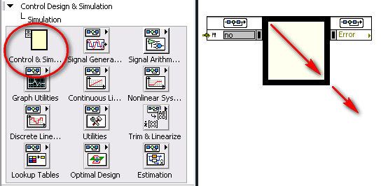
Figure 1. Create a Control & Simulation Loop.
Again on the Simulation subpalette, select Continuous Linear Systems and click once on Transfer Function and once inside the Control & Simulation Loop you created previously. This places a Transfer Function block inside the Control & Simulation Loop. Now double-click on the Transfer Function block to input the transfer function parameters.

Figure 2. Select a Transfer Function.
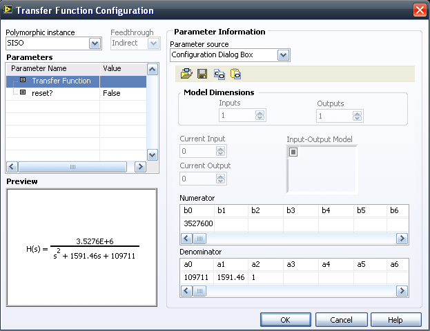
Figure 3. Input Transfer Function parameters.
Now implement the PID algorithm. On the function palette, select the Control Design & Simulation->PID subpalette and drag and drop the PID.vi into the Control & Simulation Loop. Because the PID algorithm is going to run on a Real-Time based operating system with a fixed loop rate, right-click on the PID.vi and select SubVI Node Setup…. to bring up a configuration dialog window. You can use this window to configure the simulation loop to handle timing with this particular VI. Assume the controller is going to run at a 1000 Hz loop rate, so select discrete with a period value of 0.001 seconds.
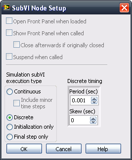
Figure 3. PID subVI configuration for timing inside the Control & Simulation Loop.
The “D” that appears on the PID VI indicates that it is being handled as a discrete system.
Run the cursor over the PID VI until you are on top of the PID Gains Terminal (you might type CTRL+H to Show Context Help if you cannot find it). Right-click and select Create->Control. This creates a control on the Front Panel that you can use to change the PID gains interactively. Finally, right-click on the dt(s) terminal and create a constant. This should be the same as the digital period you created previously, 0.001 seconds.
To create an input signal, use a step signal. From Control Design & Simulation->Simulation->Signal Generation, select Step Signal and drop it into the simulation loop. Leave parameters as they are configured by default.
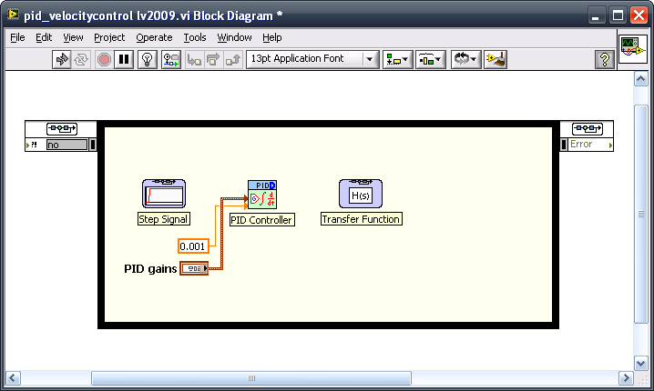
Figure 4. Create an input signal using a step signal.
Now create the components necessary to view the simulation results. First bundle the input (Step Signal) with the output from the motor transfer function into a Build Array node, which you can find on the Programming->Arrays subpalette. Collect these signals and plot them on a graph on the Front Panel. To do so, select Control Design & Simulation->Simulation->Utilities then select and drop Collector. On the Front Panel, create an XY Graph to display the simulation results. Connect all the signals as shown in Figure 5.
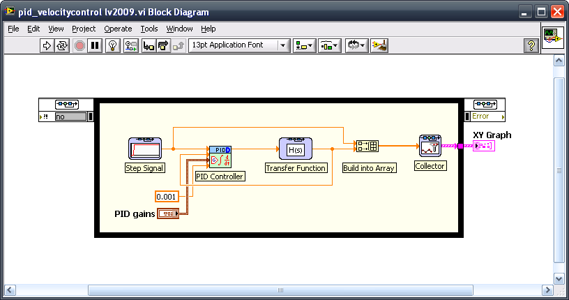
Figure 5. Collect the signals.
If you rearrange the Front Panel elements and use the default values, you will end up with a graph similar to Figure 6:

Figure 6. View the simulation results graphically.
Fine-Tune the Simulation
Use LabVIEW native graphical capabilities to improve the simulation and fine-tune the PID gains.
First, change axis properties to have a better view of the simulation results. Right-click on the border of the XY Graph and uncheck the AutoScale X property under the X Scale option.
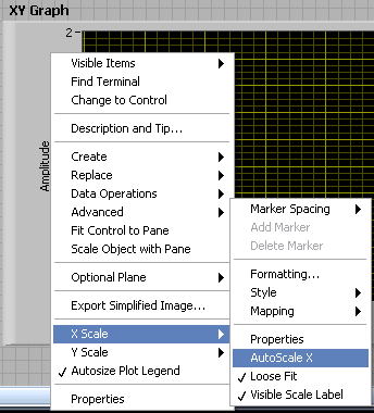
Figure 7. Graph properties.
Before making changes to the PID controller, we will make the simulation more efficient. As seen on Figure 6 there is no need to simulate the default 10 seconds; the plant is fast enough so that a final simulation time of 2 seconds is enough. Now modify the simulation parameters by double-clicking on the Control & Simulation Loop configuration pane which calls up the Configure Simulation Parameters dialog window. Implement the parameters as shown in Figure 8.
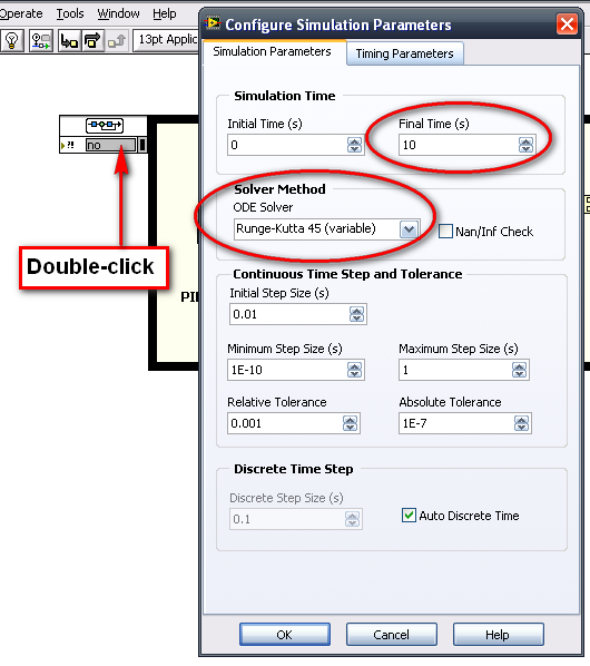
Figure 8. Change the simulation parameters.
PID Tuning
You now can run the VI continuously and change the PID gains until you are satisfied with the results.
A typical procedure to tune a PID controller would be:
- Kc to 1 and Ti, Td to zero. Keep increasing/decreasing Kc until the response has some overshoot
- Modify Td to make the system faster and compensate the overshoot
- Modify Ti to remove any steady-state error on the step response
See Simple Servo Motor Tuning and finding PID gains for more information on tuning a PID controller.
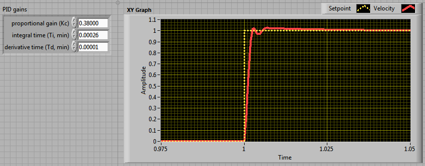
Figure 8. Simulation results with Kc=0.38, Ti=0.00026, and Td=0.0001.
Conclusion
You now know how to simulate a discrete-based PID controller with the continuous dynamic system behavior of a DC motor. You can apply this technique to any kind of hybrid system where continuous and discrete behavior is mixed. One of the benefits of the procedure shown is that the control algorithm you used is exactly the same as the one you would use in a Real-Time implementation, and you can take advantage of many of its features, such as integral anti-windup.