Configuring a Fourier Analysis in Multisim

Multisim features a comprehensive suite of SPICE analyses for examining circuit behavior. These analyses range from the basic to sophisticated. Each analysis helps you to obtain valuable information such as the effects of component tolerances and sensitivities. For each analysis, you need to set settings that will inform Multisim exactly what to analyze, and how.

Multisim simplifies the procedure for an advanced analysis by providing a configuration window. This abstracts away the complexities associated with SPICE syntax and configuration of analysis. With this window, you merely need to specify the parameter values and output nodes of interest.

This tutorial is part of the NI SPICE Analysis Fundamentals Series. Each tutorial in this series provides you with step-by-step instructions on how to configure and run the different SPICE analyses available in Multisim.powerful simulation and analysis while abstracting the complexity of SPICE syntax.

Introduction

Fourier Analysis is a method of analyzing complex periodic waveforms. It permits any nonsinusoidal period function to be resolved into sine or cosine waves, possibly an infinite number, and a DC component. This permits further analysis and allows you to determine the effect of combining the waveform with other signals.

Given the mathematical theorem of a Fourier series, the period function f(t) can be written as follows:

f(t) = A₀ + A₁cosωt + A₂cos2ωt + … + B₁sinωt + B₂sin2ωt + …

where:

A₀ = The DC component of the original wave.

A₁cosωt + B₁sinωt = The fundamental component (has the same frequency and period as the original wave).

A_ncosnωt + B_nsinnωt = The n^th harmonic of the function.

A, B = The coefficients.

ω = 2¶/T = The fundamental angular frequency, or 2π times the frequency of the original periodic wave.

Each frequency component (or term) of the response is produced by the corresponding harmonic of the periodic waveform. Each term is considered a separate source. According to the principle of superposition, the total response is the sum of the responses produced by each term. Note that the amplitude of the harmonics decreases progressively as the order of the harmonics increases. This indicates that comparatively few terms yield a good approximation.

When Multisim performs Discrete Fourier Transform (DFT) calculations, only the second cycle of the fundamental component of a time-domain or transient response (extracted at the output node) is used. The first cycle is discarded for the settling time. The coefficient of each harmonic is calculated from the data gathered in the time domain, from the beginning of the cycle to time point t. That is set automatically and is a function of the fundamental frequency. This analysis requires a fundamental frequency matching the frequency of the AC source or the lowest common factor of multiple AC sources.

Fourier Analysis produces a graph of Fourier voltage component magnitudes and, optionally, phase components versus frequency. By default, the magnitude plot is a bargraph but may be displayed as a line graph.

The analysis also calculates Total Harmonic Distortion (THD) as a percentage. The THD is generated by notching out the fundamental frequency, taking the square root of the sum of the squares of each of the n harmonics, and then dividing this number by the magnitude of the notched out fundamental frequency:

THD = [ (S_i=2V_i²)/V₁] x 100%

where V_i is the magnitude of the i^th harmonics.

 

Running Fourier Analysis

Consider the triangle-wave generator shown in Figure 1. This circuit generates a triangular waveform with a frequency of about 1 kHz; the circuit was taken from [1]. You will use Fourier Analysis to determine its frequency spectrum.  

Figure 1. Triangle-wave generator.
 

Complete the following steps to configure and run a Fourier Analysis:

1. Open circuit file triangle_wave.ms11 located in the Downloads section.
2. Open the Oscilloscope front panel and run the simulation. Observe the output of the circuit.
3. Stop the simulation.
4. Select Simulate»Analyses»Fourier Analysis. The Fourier Analysis window opens.Table 1 describes the Analysis Parameters tab in detail.

Table 1. Parameters used in Fourier Analysis.

Parameter	Meaning
Frequency resolution (Fundamental frequency)	Sets the frequency of an AC source in your circuit. If you have several AC sources, use the lowest common factor of frequencies. Click the Estimate button to have the fundamental frequency estimated.
Number of harmonics	Sets the number of harmonics of the fundamental frequency that are calculated.
Stop time for sampling (TSTOP)	Sets the amount of time during which sampling should occur. You can specify this value to avoid unwanted transient results prior to the circuit reaching steady-state operation.
Edit transient analysis	Displays the Analysis Parameters tab of the Transient Analysis window. The analysis will use either the Maximum time step (TMAX) and Set initial time step (TSTEP) values that you enter in this tab, or an automatically calculated minimum value that is based on the value in the Frequency resolution (Fundamental frequency) field in the Analysis Parameters tab of the Fourier Analysis window—whichever offers a higher sampling rate (resulting in a more accurate simulation).
Display phase	Displays phase results.
Display as bar graph	Displays results as bar graph. If not enabled, results are displayed as linegraph.
Normalize graphs	Normalizes graphs against the 1st harmonic.
Display	Choose a display option: Chart, Graph, or Chart and Graph.
Vertical Scale	Choose a vertical scale: Linear, Logarithmic, Decibel, or Octave.
Degree of polynomial for interpolation	Enable to enter degree to be used when interpolating between points on simulation. The higher the degree of polynomial the greater the accuracy of the results.
Sampling frequency	Specifies a sampling frequency. This value should be equal to the frequency resolution (the number of harmonics plus one) multiplied by at least 10.

Note: In SPICE, the command that performs a Fourier Analysis has the following form:

.FOUR FREQUENCY OUTPUT_SPECIFICATION <OUTPUT_SPECIFICATION …>

Where .FOUR initializes a Fourier Analysis; FREQUENCY specifies the fundamental frequency of the transient waveform to be analyzed; OUTPUT_SPECIFICATION specifies the quantity to be reported as the result of the Fourier Analysis. Note that these parameters are similar to those defined in Table 1, however, in Multisim you do not have to worry about the SPICE syntax.  
 

5. Configure the Analysis Parameters as shown in Figure 2.

Figure 2. Analysis Parameters for the Fourier Analysis.
 

6. Click the Edit transient analysis button.
7. Configure the Transient Analysis window as shown in the following figure:

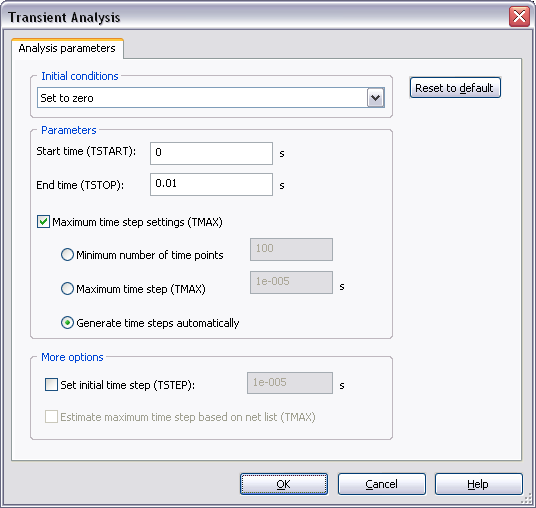
Figure 3. Transient Analysis window.

For more details on how to configure the Analysis Parameters tab refer to the Transient Analysis  tutorial.

8. Click OK.
9. Select the Output tab.
10. Select the Variables in circuit list, select Static Probes from the drop-down list, and then highlight V(Probe1) from the list.
11. Click the Add button to move the variable to the right side under Selected variables for analysis, as shown below.

Figure 4. Output variable for the Fourier Analysis.
 

12. Click Simulate. The Grapher View window opens. Results are displayed in Figure 5.

Figure 5. Fourier Analysis results.
 

As you can see, results are divided in two parts: the chart lists detailed information including the DC component and THD; the graph show the frequencies and their magnitudes. You can use the Cursors to take precise measurements.

 

References

[1] OP-AMP Circuits and Principles, Howard M. Berlin, Sams Publishing, 1991, ISBN 0-672-22767-3.