Configuring a Parameter Sweep Analysis in Multisim

Multisim features a comprehensive suite of SPICE analyses for examining circuit behavior. These analyses range from the basic to sophisticated. Each analysis helps you to obtain valuable information such as the effects of component tolerances and sensitivities. For each analysis you need to set settings that will inform Multisim exactly what to analyze, and how.

Multisim simplifies the procedure for an advanced analysis by providing a configuration window. This abstracts away the complexities associated with SPICE syntax and configuration of an analysis. With this window you merely need to specify the parameter values and output nodes of interest.

This tutorial is part of the SPICE Analysis Fundamentals Series. Each tutorial in this series provides you with step-by-step instructions on how to configure and run the different SPICE analyses available in Multisim, powerful simulation and analysis while abstracting the complexity of SPICE syntax.

Introduction

The behavior of a circuit is affected when certain parameters in specific components change. With Parameter Sweep Analysis, you can verify the operation of a circuit by simulation across a range of values for a component parameter. The effect is the same as simulating the circuit several times, once for each value. You control the parameter values by choosing a start value, end value, type of sweep that you wish to simulate and the desired increment value. There are three types of analysis that can be performed on the circuit while the component is manipulated: DC Operating Point, Transient Analysis  and AC Analysis.

You will find that some components have more parameters that can be varied than others. This will depend on the model of the component. Active components such as op-amps, transistors, diodes and others will have more parameters available to perform a sweep than passive component such as resistors, inductors and capacitors. For example the inductance is the only parameter available for an inductor as compared to a diode  model that contains approximately 15 to 25 parameters.

Running Parameter Sweep Analysis

Consider the series RLC circuit shown in Figure 1. According to the theory the characteristic equation modeling this circuit can be represented as:

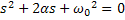
Where α is the damping factor and ω₀  the natural frequency (or resonant frequency). They are defined by:

From the above equations you can see that as the value of R increases α increases and the RLC circuit is driven towards an overdamped response since the value of α in relation to ω₀ determines the behavior of the circuit’s response. There are three possible responses:

• α < ω₀ : Underdamped response
• α = ω₀ : Critically damped response
• α > ω₀ : Overdamped response

In this example you will use Parameter Sweep Analysis to plot the transient step responses of the RLC circuit when R is varied.

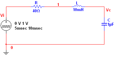
Figure 1. Series RLC circuit.

 

Complete the following steps to configure and run a Parameter Sweep Analysis:

1. Open circuit file series_rlc_circuit.ms11 located in the Downloads section.
2. Select Simulate»Analyses»Parameter Sweep. The Parameter Sweep window opens. Table 1 describes the Analysis Parameters tab in detail.

 

Table 1. Parameters used in Parameter Sweep Analysis.

Parameter	Meaning
Sweep Parameter	Select a sweep parameter by choosing a parameter type (Device  or Model) from the Sweep Parameter drop-down list, then enter information in the Device Type, Name, and Parameter fields.  A brief description of the parameter appears in the Description field and the present value of the parameter is displayed in the Present Value field.
Sweep Variation Type	Dictates how to calculate the interval between the start and stop values. Parameter Sweep Analysis plots the appropriate curves sequentially. The number of curves is dependent on the type of sweep as shown below: Decade: The number of curves is equal to the number of times the start value can be multiplied by ten before reaching the end value.   Linear: The number of curves is equal to the difference between the start and end values divided by the increment step size. Octave: The number of curves is equal to the number of times the start value can be doubled before reaching the end value. List: The number of curves is equal to the number of values entered in the Value List (items in the list must be separated by spaces, commas or semicolons).
Analysis to sweep	Select the analysis to sweep. There are four options: DC Operating Point AC Analysis Transient Analysis Nested Sweep You can set the analysis parameters by clicking the Edit Analysis button.

 

3. Configure the Analysis Parameters tab as shown in Figure 2.  

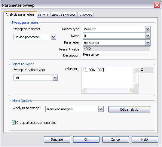
Figure 2. Analysis parameters for the Parameter Sweep Analysis.

Note that in this case the analysis will sweep the parameter R (resistance) using the following values: 40 W, 200 W and 1 kW, therefore, three curves will be generated.

4. Click on the Edit Analysis button. The Sweep of Transient Analysis window opens.
5. Configure the Analysis Parameters as shown in the following figure:

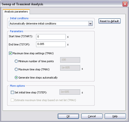
Figure 3. Sweep of Transient Analysis window.

Refer to the Transient Analysis tutorial for more details on how to configure the Analysis Parameters tab.

6. Click OK to close the Sweep of Transient Analysis window.
7. Select the Output tab.
8. Select the Variables in circuit list, select All variables from the drop-down list, and then highlight V(c) from the list.
9. Click the Add button to move the variable to the right side under Selected variables for analysis, as shown below.

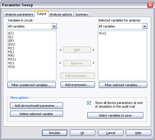
Figure 4. Output variable for the Parameter Sweep Analysis.

 

10. Click Simulate. The Grapher View window opens and plots the three typical step responses of the RLC circuit (Figure 5).

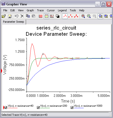
Figure 5. Parameter Sweep Analysis results.

 

11. Close the Grapher View.
12. Configure and run a Parameter Sweep Analysis with a linear sweep from 40 Ω to 1 kΩ. See Figure 6 for more details.

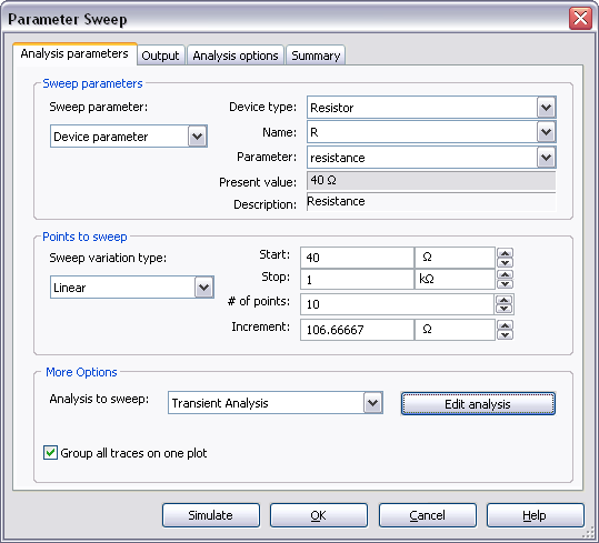
Figure 6. Parameter Sweep Analysis settings for a linear sweep.

 

You can also perform nested sweeps, combining various levels of device/model parameter sweeps.