Configuring an AC Analysis in Multisim

Multisim features a comprehensive suite of SPICE analyses for examining circuit behavior. These analyses range from the basic to sophisticated. Each analysis helps you to obtain valuable information such as the effects of component tolerances and sensitivities. For each analysis you need to set settings that will inform Multisim exactly what to analyze, and how.

Multisim simplifies the procedure for an advanced analysis by providing a configuration window. This abstracts away the complexities associated with SPICE syntax and configuration of an analysis. With this window you merely need to specify the parameter values and output nodes of interest.

This tutorial is part of the NI SPICE Analysis Fundamentals Series. Each tutorial in this series provides you with step-by-step instructions on how to configure and run the different SPICE analyses available in Multisim.powerful simulation and analysis while abstracting the complexity of SPICE syntax.

1. Introduction

AC Analysis is used  to calculate the small-signal response of a circuit. In AC Analysis, the DC operating point is first calculated to obtain linear, small-signal models for all nonlinear components. Then, the equivalent circuit is analyzed from a start to a stop frequency. The result of an AC Analysis is displayed in two parts: gain versus frequency and phase versus frequency.

Multisim performs AC Analysis using the following process:

1. DC operating Point Analysis is performed to obtain the small-signal models.
2. A complex matrix, containing both real and imaginary components is created. Multisim constructs this matrix using the following approach:

• DC sources are given zero values.
• AC sources, capacitors, and inductors are represented by their AC models.
• Nonlinear components are represented by linear AC small-signal models, derived from the DC operating point solution.
• All input sources are considered to be sinusoidal, their frequency is ignored.
• If the Function Generator is set to a square or triangular waveform, it will automatically switch internally to a sinusoidal waveform.

3. AC circuit response is calculated as a function of frequency.

Assumptions: The analysis is applied to an analog circuit, small-signal. Digital components are treated as large resistances to ground.

 

2. Running AC Analysis

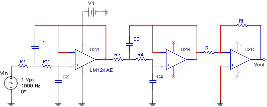
Consider the circuit shown in Figure 1. This is a fourth-order Butterworth low-pass filter with a cutoff frequency of 500 Hz and a passband gain of 10 (20 dB); this circuit was taken from [1]. You will use AC Analysis to determine its frequency response.  

Figure 1. Butterworth low-pass filter.

 

Complete the following steps to configure and run an AC Analysis:

1. Open circuit file butterworth_filter.ms11 located in the Downloads section.
2. Open the Oscilloscope front panel and run the simulation.  
3. Stop the simulation and change the frequency of the AC_VOLTAGE source, Vin.  Experiment with different values to see the circuit’s behavior. The circuit will attenuate frequencies greater that 500 Hz.
4. Stop the simulation.

If you want to perform the analysis with specific values for magnitude and phase, double-click the input source, Vin, go to the Value tab and enter values for AC Analysis Magnitude and AC Analysis Phase. In this exercise you will use the default values, 1V and 0°, respectively. The additional settings in the Value tab are used for other analyses or for simulating with the instruments.

5. Select Simulate»Analyses»AC Analysis. The AC Analysis window opens. Table 1 describes the Frequency Parameters tab in detail.

Table 1. Parameters used in AC Analysis.

Parameter	Meaning
Start frequency (FSTART)	Starting frequency of the frequency sweep. It must be greater than zero.
Stop frequency (FSTOP)	Ending frequency of the frequency sweep. It must be greater or equal to the starting frequency.
Sweep Type	Indicates how the analysis frequency is swept. There are three options: Decade: Log sweep, by decades. Octave: Log sweep, by octaves. Linear: Linear sweep.
Number of points per decade	Number of points in the sweep. Its interpretation depends on the Sweep Type. For Decade/Octave, is the number of points per decade/octave. For Linear, is the total number of points spaced evenly from the start to the stop frequency.
Vertical scale	Controls the y-axis scaling on the output graph.

Note: In SPICE, the command that performs an AC Analysis has the following form:

.AC <F_SWEEP> <POINTS> <F_START> <F_STOP> 

Where .AC initializes an AC Analysis; <F_SWEEP> is the sweep type; <POINTS> is the number of points in the sweep; <F_START> and <F_STOP> are the start and stop frequencies respectively. Note that these are the same parameters that were defined in Table 1, however, in Multisim you do not have to worry about the complex SPICE syntax.  

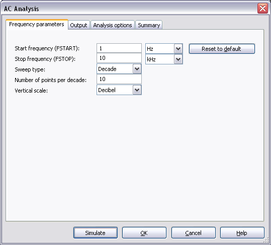
6. Configure the Frequency Parameters as shown in Figure 2. You can reset all the parameters to their default values by clicking the Reset to default button.

Figure 2. Frequency parameters for the AC Analysis.

The parameters shown in Figure 2 will perform an AC Analysis with frequency sweep from 1 to 10,000 Hz with four subintervals: 1 to 10, 10 to 100, 100 to 1,000, and 1,000 to 10,000. Each subinterval will have 10 points. The greater the number of points calculated, the more accurate the results will be.

7. Select the Output tab.
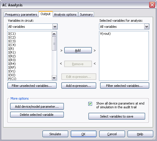
8. Select the Variables in circuit list, select All variables from the drop-down list, and then highlight V(out) from the list.
9. Click the Add button to move the variable to the right side under Selected variables for analysis, as shown below:

Figure 3. Output variable for the AC Analysis.

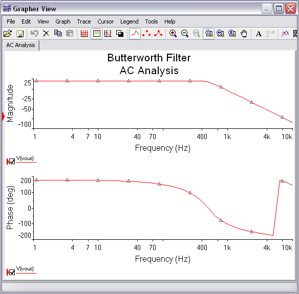
10. Click Simulate. The Grapher View window opens. Results are displayed in Figure 4.

Figure 4. AC Analysis results.

11. Select View»Show Cursors. On the left side of the Magnitude plot you will see a set of cursors. Click one of them, drag it to the right and observe the changes on the cursor information dialog. You can use cursors to take precise measurements.

An additional example file, low_pass_filters.ms11, can be found in the Downloads section. This file contains two subcircuits: a fourth-order low-pass filter in cascade and the Butterworth filter used in the previous exercise. Run AC Analysis to compare their magnitude responses.

 

References

[1] Electric Circuits, James W. Nilsson, Pearson Prentice Hall, 2005, ISBN 0-13-146592-9.