1. Vector Signal Analyzers
Vector signal analyzers (VSAs) are a popular choice for analyzing modern communication systems because of the advantages they offer over traditional spectrum analyzers. As the name suggests, VSAs are able to perform not only scalar spectral analysis but also complex time domain analysis and demodulation critical for many applications.
When considering spectral analysis alone, FFT-based VSAs offer advantages over traditional swept spectrum analyzers as well. Traditional swept analyzers work well for stable signals but for transient and bursted signals the swept nature can result in only analyzing the period of interest for a portion of the acquired spectrum. In contrast, because FFT-based VSAs acquire data for all frequencies simultaneously, the entire calculated spectrum can represent the same period of interest. FFT-based VSAs also have significantly reduced measurement times when using a narrow resolution bandwidth (RBW). Unlike a traditional swept analyzer, the VSA does not have to wait for an analog filter to settle as the LO is swept across the entire frequency span.
Although FFT-based VSAs offer many benefits, it can still be important to correlate settings to those of traditional spectrum analyzers. When there is no direct correlation between the two architectures, some form of emulation is required. Video Bandwidth (VBW) and detectors are such settings examined further in this document.
2. VBW and Detectors in a Traditional Swept Spectrum Analyzer
VBW – When measuring signals in the presence of noise, it is useful to be able to reduce the variation in the noise as much as possible while leaving the signal of interest unaffected. On traditional swept spectrum analyzers, you can use the video filter for this purpose. On traditional spectrum analyzers, the video filter is a physical low pass filter that is present in the path between envelope detection and digitizing of the signal. As the adjustable bandwidth is lowered beyond the RBW filter bandwidth, the filter reduces fluctuations in the signal (noise levels) resulting in a smoothed appearance. However, any stationary portions of the signal, for example, tones, are left unchanged.
The following two figures illustrate the qualitative effect of VBW on the displayed spectrum. Figure 1 shows a spectrum of a signal without any video filtering.
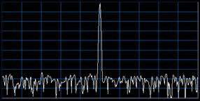
Figure 1. Spectrum trace without video filtering
Figure 2 shows the spectrum of the same signal but with video filtering applied. The reduction in noise variation is clear when you compare the two spectrums.
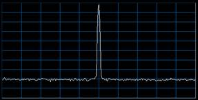
Figure 2. Spectrum trace with video filtering applied
Detectors – When you want to determine what values should represent the measured spectrum on a display with a fixed number of points, you must choose some algorithm. In traditional swept spectrum analyzers, detectors serve this purpose. The detector reduces intervals of continuously swept data down to discrete display points across both time and frequency. In terms of the frequency, the detector reduces the data contained in an interval defined by [Span]/[Number of display points] to a single display point. In terms of time, the detector reduces the data contained in an interval defined by [Sweep Time]/[Number of display points] to a single display point. The value chosen to represent the interval is determined by the type of detector chosen, for example, the average of the data in the interval, the positive peak of the data in the interval, and so on.
Note: The number of display points is user-configurable on many traditional spectrum analyzers but this doesn’t change the general premise behind detectors. The application of detectors is still a mapping process – the user can simply choose the number of points in the resulting map.
Figure 3 illustrates the application of a peak detector. The image on the left represents the continuous signal and the image on the right represents the points on the display. In this case, the maximum value in each of the 5 intervals on the left is chosen to represent the entire interval. Each of these values is then mapped as a single point on the display to the right.
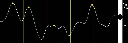
Figure 3. A continuous signal representation on the display when using a maximum peak detector
3. Emulating VBW
Spectrum – Because no VBW filter is present in the hardware architecture for VSAs, you must emulate the behavior in the software. One possible approach attempts to emulate the swept behavior of traditional analyzers by shifting the frequency in a sweep-like fashion and then applying both an RBW and VBW filter to the time domain (I/Q) data. However, this approach doesn’t utilize the advantages of FFT-based VSAs mentioned previously . Instead of this approach, this section of the document explores mathematical equivalents that leverage FFT-based analysis.
One such approach is to perform averaging on multiple acquired spectrums. From a conceptual standpoint this makes sense, because trace averaging reduces noise levels and smooths the trace –analogous to VBW.
To emulate the action of the traditional VBW filter, you must ensure that the number of acquisitions averaged results in the expected amount of reduction in the standard deviation of the spectral power of random noise signals. It is well established that the standard deviation of the average of N independent random samples is reduced to the standard deviation of the samples themselves divided by square root of N. Furthermore, when the VBW is significantly lower than the RBW, the standard deviation of the noise power measurements is reduced by approximately the square root of the ratio of the equivalent noise bandwidth (ENBW) of the envelope-detected RBW filter response to the ENBW of the video filter response. So, at least in the limit, where RBW/VBW is high, the required number of averages N to have the same effect as the VBW filter is equal to the ratio of the ENBWs of the baseband-detected RBW filter response and the video filter response.
The ENBW of the video filter is simple to calculate. Usually the traditional analog VBW filter is a simple first-order lowpass filter, having a single pole at the nominal frequency of the filter. Assuming this filter, the ENBW is π/2 multiplied by the nominal VBW frequency.
The ENBW of the detected RBW filter response is more complicated. In a traditional analog spectrum analyzer, the signal, noise in this case, is effectively fed through a bandpass filter centered at the corresponding frequency on the x-axis of the spectrum display and having a –3 dB bandwidth equal to the nominal RBW. The power of the noise making it through the filter is then measured; this measured power exists as a continuous-time signal inside an analog instrument and is further filtered by the video filter. However, while the RBW filter operates on IF signals, the nonlinear process of detecting power relocates the signal energy from IF to baseband. The spectrum of this noise energy is no longer shaped like the bandpass filter spectrum occurring before the envelope detector. This spectral transformation for power detection was characterized by S. O. Rice in 1944, when he showed that the resulting power spectrum was the same as the original narrowband power spectrum convolved with itself in the frequency domain,except at f = 0.
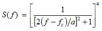
The typical analog spectrum analyzer uses 4thorder synchronously-tuned bandpass filters as RBW filters. Ideally the magnitude response is described using the following equation:
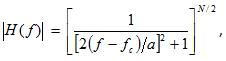
where  is the passband center frequency,
N is the order of the filter, in this case, 4,
and B is the -3 dB bandwidth of the RBW filter.
When white noise is passed through the filter, the normalized power spectrum becomes:
When the signal is detected by a square-law detector or any other detection that indicates power, Rice’s convolution indicates that the resulting spectrum will be:
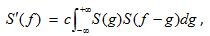
where the constant c will not matter for the calculation of ENBW, because ENBW is, in turn, calculated using the following equation:
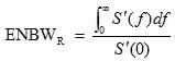
When the detected ENBW is calculated numerically for the 4th-order bandpass filter, the result is:
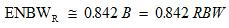
And, because ENBW is π/2 multiplied by the nominal VBW frequency , we know the ENBW of the video filter is:

Hence for VBW << RBW,

However, this approximation for N is not accurate when VBW is not much less than RBW or is greater than RBW. For example when VBW >> RBW, the video filter has almost no effect at all, and the number of averages N should be unity. Instead, the previous formula results in a very small number, much less than unity. To solve this problem, you need a function that interpolates between unity at one end and 0.536(RBW/VBW) at the other. The following function provides a good approximation of the theoretical number of averages for any RBW / VBW ratio:
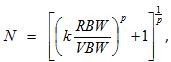
where k = 0.536 and p = 1.275.
Figure 4 illustrates how well this function approximates the ideal number of averages for all RBW / VBW ratios.
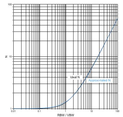
Figure 4. Function approximating ideal number of averages based on RBW/VBW ratio
Zero Span – In zero span mode, you can perform a more direct emulation because you are operating in the time domain with (I/Q) data. In this case, you can simply implement the first order video filter in software using the following impulse response equation:
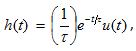
where
Note: When applying VBW, the unit of the data on which the algorithm is performed affects the overall result. In the case of both spectrum and zero span, the NI-RFSA Soft Front Panel (SFP) applies the algorithm on linear power data, that is,  . The final display unit is applied later as a post processing step. This is consistent with trace averaging, which is always applied on linear power data.
4. Emulating Detectors
To emulate detectors in the SFP, it is useful to revisit their purpose -to reduce data for display.
Frequency – As described previously, in swept analysis the reduction is defined by the ratio of Span to Number of display points. FFT analysis adds a third variable, RBW. The number of points returned by the FFT is a result of the Span, RBW, and RBW type settings. For large Span to RBW ratios, the size of the FFT can become very large. One possible method to reduce the large dataset returned by the FFT is to specify a smaller, fixed number of data points. The detector type specifies the way in which the display points are chosen from the original dataset.
In the case of the NI-RFSA SFP, the number of display points is not specified. Instead, the number of display points is equal to the size of the FFT, calculated based on the configured Span and RBW. Although it may be hard to distinguish all points on the graph for large FFTs, all the points are available for measurements, markers, exporting of data, and so on. So in the case of the SFP, detectors are not applied across frequency but are only applied over time as described in the following section.
Time – In FFT analysis, the acquisition time necessary to compute a single spectrum is predominantly dictated by the values for RBW and VBW. If you specify a sweep time greater than the acquisition time, you can perform multiple acquisitions to capture spectral information over the requested interval. In this case, you must reduce multiple acquisitions down to a single spectrum to view on the display. The detector type specifies the way in which this reduction occurs.
In the case of the NI-RFSA SFP, because sweep time is not currently a configurable parameter, the SFP uses an “auto sweep time” to provide the best correlation with the default sweep time settings of traditional analyzers . This sweep time dictates a number of acquisitions for which the SFP calculates corresponding spectrums. These multiple spectrums are reduced to a single spectrum with the detector being applied on each frequency bin.
For example, assume that the sweep time specifies to calculate two spectrums and the detector is set to peak. In this case, for the first frequency bin, the value chosen for display on the graph by the SFP is the maximum of the value of the first frequency bin of the first spectrum and first frequency bin of the second spectrum. The value chosen for display on the graph by the NI-RFSA SFP for the second frequency bin is the maximum of the value of the second frequency bin of the first spectrum and the second frequency bin of the second spectrum. The remaining frequency bin values are calculated in a similar fashion.
Optimization – For fastest measurement results in the NI-RFSA SFP, use the default detector setting, which is Sample. Sample detector can represent any point in a given interval as long as it is consistently chosen across intervals. As such, the SFP chooses the first point in the interval to be the representative sample and subsequently skips any unnecessary additional acquisitions.