Solution
The
Simulate Signal Express VI allows you to create a waveform according to a number of different parameters like frequency and amplitude. Subtle changes in many of the timing parameters can have major implications in the waveform. The following list explains how each of the parameters affect the waveform.
- Samples Per Second and Number of Samples—Even though you can specify the frequency of your waveform using the Signal options in the dialog box, Samples per second (Hz) and Number of samples determine how LabVIEW represents the frequency and over what range of data points the frequency occurs. For example, if you leave all values as default in the configuration window, the frequency will be 10.1 Hz, with 1000 samples per second and 100 samples. This implies that 100 data points will be output to generate a waveform (sine, by default) with a frequency of 10.1 Hz. The dataset that appears will contain points that span .1 seconds, as dictated by our 1000 samples per second requirement with 100 samples. The following equation helps clarify this:
Seconds of Data = Number of Samples/Samples per Second
To receive a full second worth of data, we would need to change the number of samples to 1000. This would yield a dataset with 10.1 cycles of a sine wave spanning that dataset.
- Integer Number of Cycles—If you are going to be calling the Simulate Signal Express VI in a loop or sending the output waveform to an analog output buffer, you will probably want the dataset to appear continuous over multiple iterations or output operations. Using the example from above, a 10.1 Hz sine wave contains 10.1 cycles in a second. This leaves the end of our dataset with somewhere in the middle of the last sine wave cycle. If you loop this dataset repeatedly, you will see a discontinuity as the dataset jumps from the middle of our last sine wave to the beginning of the first sine wave in the next call. This discontinuity can be especially troublesome in continuous analog output operations. To overcome this, place a checkmark in the Integer number of cycles checkbox to make sure the output waveform does not end in the middle of cycle. This ensures the next cycle picks up from where the previous one stopped.
Note: When only an integer number of cycles is allowed, the frequency you specify may not be attainable in the number of samples you set to output. Consequently, the Simulate Signal Express VI recalculates the appropriate number of samples to output that achieves the desired frequency, or close to it, in an integer number of cycles. If the actual frequency is not close enough to the frequency you specify in an integer number of cycles, increase the number of samples by removing the checkmark for the Automatic checkbox to change the number of samples.
- Reset Signal—While Integer number of cycles ensures no discontinuities for a continuous waveform, it has been noted that achieving the exact frequency can be difficult when you use that option. If a continuous waveform is desired at a very precise frequency, select Use continuous generation from the Reset Signal options in the Simulate Signals Express VI dialog box. The Simulate Signal Express VI will retain information from its previous call if you call it multiple times. This allows some seeding information to be planted into subsequent calls, removing the possibility of discontinuities. This option is the best method for continuous generation from the Simulate SignalExpress VI.
You can also specifically ensure that the seeding from previous iterations is not applied by selecting Reset phase, seed, and time stamps.
- Simulate Acquisition Timing—As mentioned above, we know that at 1000 samples per second and 100 samples, we will get .1 seconds of data. By default, however, it does not take .1 seconds to generate that dataset. In reality it happens much faster (if you want to test this, try setting the parameters to 1000 samples per second and 5000 samples - it won't take 5 seconds to generate). If we select Simulate acquisition timing instead of Run as fast as possible, you will see the appropriate delay for the samples you request at the given speed. This allows you to better emulate an actual acquisition process and the timing that goes into it.
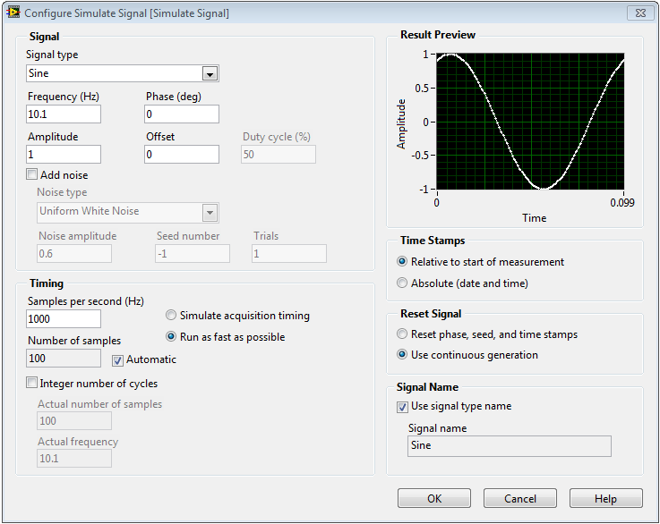
Figure 1 Simulate Signal Configuration Options
If you wire the output of the Simulate Signal Express VI directly to the data input of a DAQ AssistantExpress VI configured for continuous analog output, there are several configuration issues to keep in mind. First, as mentioned above, you may want to alleviate the possibility of any discontinuities. Second, you will NOT want to select Simulate acquisition timing because the analog output operation has the output timing built into it, so adding a delay in the generation of the waveform from the Simulate Signal Express VI could delay the output. In the DAQ Assistant Express VI that is configured for analog output, you can select the Use timing from waveform data option. This will configure the output operation to send the waveform with the timing you specified in the Simulate Signal Express VI, regardless of how quickly it is actually generated.
Refer to the LabVIEW Help for Simulate Signal Express VI for more information. Right-click the Simulate Signal Express VI on the block diagram and select Help from the shortcut menu to open the LabVIEW Help.